Site Selection of Candidate Reserve Areas in Centre, PA
Project background and objectives:
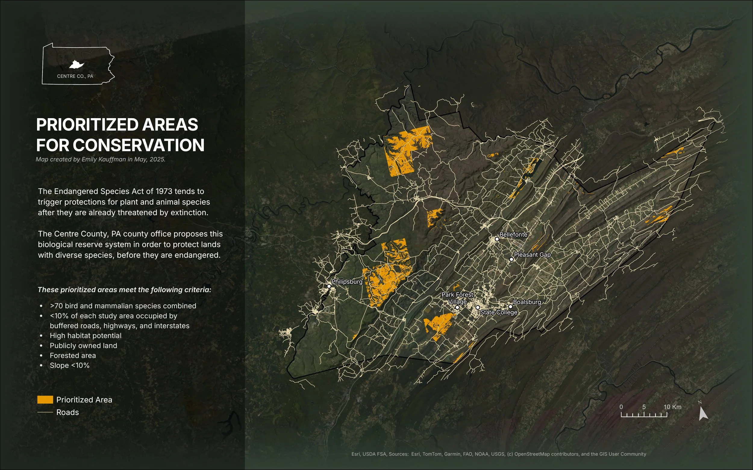
The Endangered Species Act of 1973 tends to trigger protections for plant and animal species after they are already threatened by extinction. The Centre County, PA county office has decided to propose a biological reserve system in order to protect lands with diverse species, before they become endangered (King, Walrath, & Zeiders, 1999–2026).
Criteria:
We will create a map that shows suitable study areas for protection that meet this criteria:
more than 70 bird and mammalian species combined,
less than 10% of each study area occupied by buffered roads, highways, and interstates,
high habitat potential,
publicly owned land,
is forested area,
and has a slope of less than 10% (King, Walrath, & Zeiders, 1999–2026).
Process:
The goal is to show suitable areas that meet the criteria for a potential biological reserve. To do this, we must calculate the result of each of the criteria and then combine the results to display a final map of sites.
The first step is to prepare the map and the data. I used the coordinate system NAD 1983 StatePlane Pennsylvania North FIPS 3701 (Meters). I added the provided layers: roads, study areas, ownership, habitat, boundary, landuse, and elevation, and set some initial symbology and layer ordering that makes sense for each of these. I chose a cell size of 50m because that is the coarsest cell size in the dataset (landuse layer).
Next, I went through each criteria and prepared the data.
Criteria 1: >70 bird and mammalian species combined
We are trying to find study areas that match this criteria, so I joined the studyareas layer with the standalone table, speciesrich, using the BLOCK_ID. I made a new column to hold the total richness and calculated it from the sum of the birds and mammals columns. I created a new layer from this, selecting only areas where the total richness was greater than 70.
Criteria 2: <10% of each study area occupied by buffered roads, highways, and interstates
The road data consists of typed lines (Road, Highway, and Interstate). I filtered this set down to only include roads that intersected with the high species study areas generated for criteria 1. This reduced the road areas that I would need to process, since much of it was already filtered out. I used a Python conditional statement in the Calculate Fields tool to assign a buffer distance based on the road type (Esri, n.d.-a).
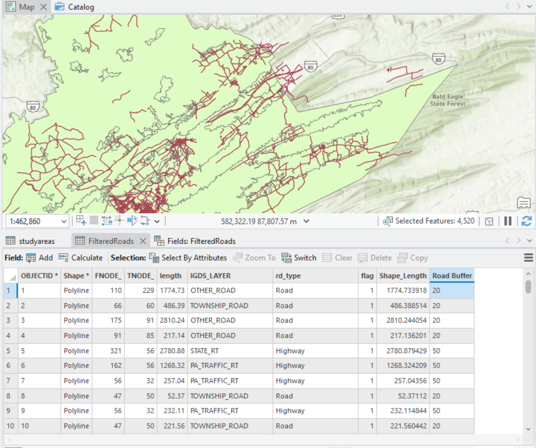
Figure 1 - This shows the FilteredRoads layer and attributes table once the Road Buffer was added. You can see that roads with a rd_type of “Road” have buffers of 20, “Highways” have 50, and although not pictured, “Interstates” have 100. These were calculated using the Python expression field in the Calculate Field tool. Image generated in ArcGIS Pro on May 1, 2026 by Emily Kauffman as part of the Lesson 9_10 project.
Since we don’t want to dissolve due to the time, instead I used the Union tool to combine the roads and their buffers with the study areas, and then only selected areas where the buffered distance was 0. This denoted the portions of each study area that were NOT roads. After dissolving by block ID, I was able to calculate both the road area and the non-road areas, and export only where the percentage was less than 10%.
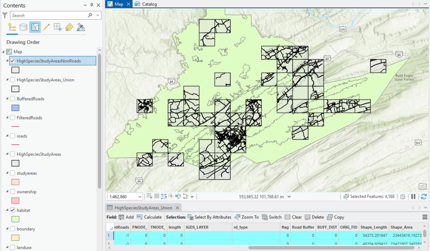
Figure 2 - This image shows the HighSpeciesStudyArea_Union attributes table and map layer. The blocks show the result of the union of 0 buffer road distances and study areas. The habitat layer is displayed in green to show the total original habitat area. Image generated in ArcGIS Pro on May 1, 2026 by Emily Kauffman as part of the Lesson 9_10 project.
Criteria 3-4: High habitat potential and publicly owned land
The habitat layer is a polygon with a habitat potential field of “High” or “Low”. We are only concerned with areas that have a high potential, so I selected by that attribute and exported to a new layer. I added a new column called “pass” to denote whether the row met the criteria, and set them all to have a value of 1. I converted this to a raster and show the areas that met the criteria. An alternative to this would have been to simply convert to a raster that included both high and low values, and then reclassify to pass or fail values based on the attribute. I followed these same steps for the publicly owned land to create a raster only showing public areas as passing.
Criteria 5: Forested area
Instead of using the pass column here, because landuse was already a raster, I simply reclassified the layer into “forest” areas (passing, value of 1), and "everything else” (failing, value of 0) that included any values that were not forest (see Figure 3).
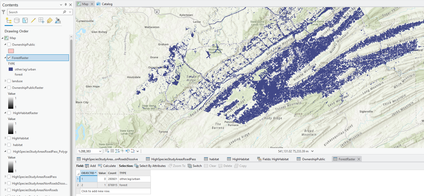
Figure 3 - This image shows the result of determining the eligible landuse area. Everything highlighted in the map is forest area, which meets the criteria. This was classified so all forest is passing criteria (value of 1) and everything else is not passing (value of 0). Image generated in ArcGIS Pro on May 2, 2026 by Emily Kauffman as part of the Lesson 9_10 project.
Criteria 6: Slope of less than 10%
To calculate the slope, I used the Slope tool with the elevation as the input raster and PERCENT_RISE as my output measurement. This created a new layer called SlopePct, which I then reclassified into areas that were less than 10% or not (see Figure 4).
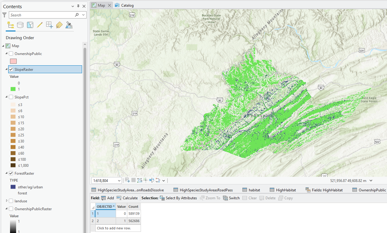
Figure 4 - This image shows the result of determining the eligible sloped area. Everything highlighted in the map is less than 10% slope, which meets the criteria. Image generated in ArcGIS Pro on May 2, 2026 by Emily Kauffman as part of the Lesson 9_10 project.
Results and Conclusions
Finally, I used the raster calculator to determine the suitable areas across the project, using the individual rasters from each of the criteria (see Figure 5). My results show that there were 51,341 cells that meet all of the criteria, and 53,020 cells that do not. Since each cell size is 50m, or 2,500m2 total, this comes out to approximately 31,716.56 acres of suitable candidate reserve areas (see Figure 5).
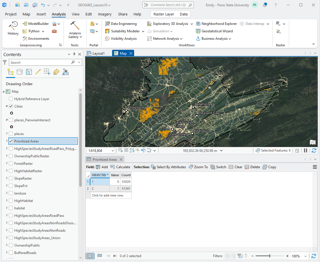
Figure 5 - This shows the final attribute table and partial map of the Prioritized Areas, generated from the raster calculator output. It shows that there are 53,020 unsuitable cells, and 51,341 suitable cells in the result. With a 50m cell size, this results in approximately 31,716.56 acres of potential reserve sites. Image generated in ArcGIS Pro on May 2, 2026 by Emily Kauffman as part of the Lesson 9_10 project.
I found it to be confusing that some of the criteria was based on the study area block, and others were not. If I were to improve on my results, I would change the criteria for how we derived an area that was not as road-heavy. In this analysis, I filtered out entire study areas that had too high of a concentration of roads, despite the fact that the roads may have been in one small area of the block. I would imagine that this removed suitable area that could have been a candidate for preservation. Also, most of the other criteria were not based on the studyareas, so this did feel arbitrary.
We were rather limited by the 50m resolution of the landuse layer. Finding a dataset with a finer resolution would have allowed for more accurate results, especially since some of the other layers were as fine as 30m.
In terms of the ecology, there are many more types of animals other than birds and mammals. I would have liked to see other creatures, or even plant diversity, factored into the results. Changing the logical criteria here would have been interesting to see. For example, how would the suitable areas change if we looked for areas that had at least thirty mammals OR fifty birds OR ten amphibians? Additionally, combining these into a total species did not take into consideration rarity of species at all. Maybe we only have two mammal species in an area, but one of them is extremely rare and should be weighted higher in the assessment.
Finally, an interesting insight that I discovered with the suitable areas is that they coincide with many existing state parks or public game lands. If I turn on a reference layer that labels these public areas, you can see the game lands and park labels appear over the orange overlay (see Figure 6). Centre County could suggest a partnership with local parks to establish these reserve areas and undertake preservation efforts together. Alternatively, it’s likely these parks have their own conservation plans in place already and we may want to exclude them from our results, since our goal is to identify suitable areas for a reserve.
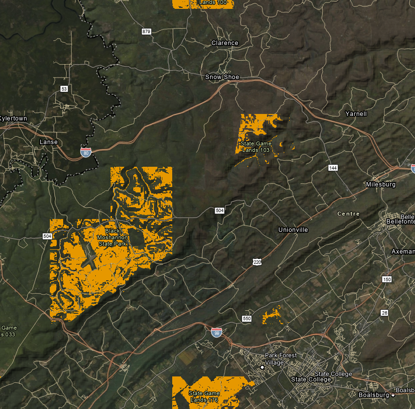
Figure 6 - This image shows a snapshot of the map with an enabled reference layer that displays state parks and game lands. You can see how the orange suitable site areas are often closely associated with these public areas. Image generated in ArcGIS Pro on May 6, 2026 by Emily Kauffman as part of the Lesson 9_10 project.
Layout:
The layout includes the hillshade layer that I derived from the elevation using the Hillshade tool, the Centre County boundary, and the roads. I included the roads and boundary layers to give the user some spatial context. This alone was not enough if you are not familiar with the area, so I added a places layer, which I filtered to only include areas with a population class of greater than four, and then displayed the labels. This allows users to tell where the suitable areas are in relation to the largest towns in Centre County. I intersected this dataset with the county boundary so that only the relevant cities would appear.
I added the Dark Gray basemap as well as the NAIP imagery basemap, and applied an overlay to NAIP. This does a great job of showing the terrain of central Pennsylvania, while keeping the overall color scheme dark and muted. I added an overlay to the hillshade layer as well so that the elevation changes come through, although there’s less emphasis. I did this so that the orange suitable area overlay would come through as the most important thematic information.
Finally, I made a map extent using the border of Pennsylvania extracted from Esri census data, and added the Centre County polygon (Esri, n.d.-b). One problem that I see here is that I have the county in the main map rotated so that it fits into the page layout better, but the map extent is not rotated. I decided that this was acceptable because there is enough information on the map to let the user know that the area of interest is Centre County, and it would be more confusing if I had also rotated the state of Pennsylvania, since that’s not how it’s normally displayed.
Figure 7 - This image shows the final layout for the lesson. It shows the suitable areas highlighted in orange, as well as the roads, and labels for a few of the more populated areas in Centre County. The map description shows the background of the project as well as the criteria used to build it. Image was generated in ArcGIS Pro on May 5, 2026 by Emily Kauffman as part of the Lesson 9_10 final project.
References:
Esri. (n.d.-a). Calculate field examples. ArcGIS Pro. Retrieved May 1, 2026, from https://pro.arcgis.com/en/pro-app/latest/tool-reference/data-management/calculate-field-examples.htm
Esri. (n.d.-b). USA States (Generalized) [Feature layer]. ArcGIS Living Atlas of the World. Retrieved May 5, 2026, from https://www.arcgis.com/home/item.html?id=d7c21ac2f29348cebf45f70515f72a42
King, E., Walrath, D., & Zeiders, M. (1999-2026). Environmental Management & Conservation, Lesson 9/10. The Pennsylvania State University World Campus Certificate/MGIS Programs in GIS. Retrieved April 28, 2026.